Estimating genomic neighbourhood with the gne module

In cblaster, the most important parameter when detecting hit clusters is the maximum inter-hit gap parameter. This determines how far cblaster will look between any two hits before terminating a given cluster. By default, this parameter is set to 20,000 bp; if no new hit is found within 20,000 bp of the previous hit in a cluster, cblaster will terminate extension of that cluster. Though the 20 kb cutoff has worked quite well for us when looking at fungi or bacteria, where gene density within clusters is quite high, it may not work for all datasets. For example, plant gene clusters may have key biosynthetic genes spread out over large stretches of the chromosome, with many genes in between; this is where the gne module comes in.

The gne module lets you robustly detect an appropriate value to use for this parameter by continually re-running cluster detection on a saved search session at different gap values over some interval. It then generates plots of the mean and median cluster sizes (bp), as well as the total number of predicted clusters, at each value. gne is run on a search sessions, like so:

$ cblaster gne session.json

And generate outputs that looks like this:

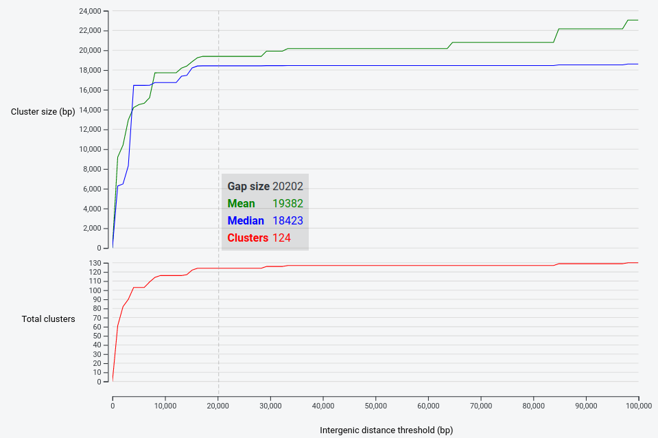
You can gain insight into the size of the given genomic neighbourhood of your query proteins – the result clusters in this case tend to be just under 20Kbp.

The gne module generates a list of gap values (total number determined by the samples parameter) from 0 to some upper limit (determined by the max_gap parameter). These numbers can be chosen in two ways. By default, gne will take evenly spaced (i.e. linear) values over the range 0-100,000 bp. Alternatively, you can choose to generate these values via a log scale, which will result in more samples at lower values than at higher ones. This can be specified using the --scale argument:

$ cblaster gne session.json --scale log

As these plots typically resemble logarithmic growth (i.e. rise steeply, then level off), it can make sense to sample more heavily in the more unstable region of the curve.

In case you would like the underlying data (e.g. for creating your own plots), gne can generate delimited output. To do this, simply use the -o or --output argument to specify a file to save the data to, and the -d or --delimiter argument to specify the delimiting character. For example, to generate a CSV file:

$ cblaster gne session.json --output gne.csv --delimiter ","

Like plots generated by the search module, gne plots can be saved as static HTML. To do this, provide a file to the -p or --plot argument:

$ cblaster gne session.json -p gne.html